
Intro
This post is the beginning of a series on “Things I wish I Understood When I Took my First Robotics Course”. The casual observer probably thinks that robotics is a lot of programming, hardware design, and general witchcraft. Valid. These things are all important to robotics, but they are not the core principles of robotics (except for maybe the witchcraft part). The foundation of robotics is in fact some really awesome math that describes how different things in space are related to each other. This (at least the part about there being lots of math) quickly becomes apparent to anyone who has cracked open a robotics textbook and discovered that it’s full of complicated looking linear algebra starting basically on page one.
My goal is to share some of my intuition with you so that you can understand at a high level what relationships that math is trying to communicate. So if you’re causally curious, an overwhelmed engineering student, or somewhere in between, join me for part 1 where we’ll introduce some fundamental concepts that we’ll build on in the rest of this series!
Trigger warning: There will be math (linear algebra) involved but don’t worry, I’ll let you know before I introduce any equations!
TLDR
There are things in math called Riemannian manifolds. These manifolds are smooth surfaces on which we use numbers to define locations in space. The manifold provides rules for how we add, subtract, multiply, divide, etc. these numbers in a semantically meaningful way.
Two examples of manifolds are a piece of graph paper and a globe. The rules for things like what distance means and what a line is are also inherent to the manifold. For example if we draw two points on the graph paper and two points on the globe, the lines that connect them will be different!
To connect our points we travel along the surface of our manifold. This means that our globe line is actually a curve while our graph paper line is what we are used to thinking of as a straight line. In reality though, these lines are both straight with respect to the surface that they were drawn on. If you were standing on the globe and walked from start to goal, you would say you had walked in a straight line even though looking at the globe our path would be more like an arc.
Whacky huh (on a separate note this is why that paths on airplane trackers always look like curves rather than straight lines, the airplane is in fact moving in a straight line but it happens to be along a curved surface…sorry, the earth isn’t flat). We call the most direct path between points along the surface a geodesic. Airplanes travel along geodesics when they fly from A to B and the line from A to B along our graph paper is also a geodesic.
How we define distance on these surfaces is a key part of the manifold. The really cool thing is that you’ve already seen an example of this! That Pythagorean theorem that you learned in middle school,
$$a^2 + b^2 = c^2$$
is actually the Riemannian distance metric for that graph paper space that we’re used to thinking about (in math we call that graph paper space Euclidian space). In robotics we use a special space called the Special Euclidean Group in 3D space or SE(3). This space has definitions for how to add, subtract, etc. positions AND rotations. At the end of the day however, SE(3) space that we use in robotics, the globe space that we were discussing, and Euclidean (graph paper) space are all Riemannian manifolds. They share similar properties and understanding the fundamentals of Riemannian manifolds will be super helpful going forward. If you want more details, keep reading! Otherwise, see you next time!
Poses and SE(3)
If you didn’t read the TLDR, please go back and read that first 🙂
The fundamental thing we do in robotics over and over again is take a position and an orientation in 3D space and figure out how to compare it to another position and orientation in 3D space. This combination of position and orientation is called a pose. In this case, a pose is not something that you strike at the end of a dance number or when someone is taking your picture. It’s actually 6 numbers that describe where you are in space and in what direction you are pointing. It’s always defined relative to something else (usually we call that something our world frame of reference) and the first three numbers describe position while the last three describe orientation/rotation.
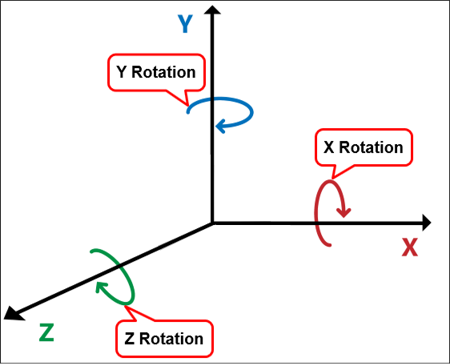
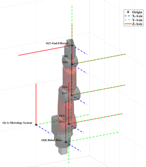
Think of a 3D graph like the one in the figure above. You have an x axis, a y axis, and a z axis. Anywhere you go in space can be defined by some combination of your x position, your y position, and your z position (i.e. your coordinates). To make it extra complicated (and extra useful) however, we also care about how your coordinate frame (i.e. the direction your axes are pointing in) is rotated around those three axes relative to the rest of the world! For example, look at the robot arm below. At each joint there is a coordinate frame that describes the pose of that joint relative to everything else. That coordinate frame at the bottom off in space is our world frame. The rest of the frames are defined relative to that. Some of them are simply translations (changes in position) relative to each other, some are simply rotations (changes in orientation) and some are both translations AND rotations (to visualize the rotations look at the directions the colors are pointing, each color represents a different axis).
This is really important because it lets us define where all the parts of our robot are relative to itself, obstacles, and things we want to interact with. As our robot moves, we can use math to update these poses and track our physical proximity to things in the world.
Poses belong to what we call Special Euclidean Group in 3D space or SE(3). Remember, our position and orientation are defined by how we move along each of the world frame axes and how we rotate relative to those axes respectively. These 6 numbers are the dimensions of our space. They are the coordinates that define everything that we need to know about where we are in the space. Here you have to stretch your brain a bit because this space is NOT 3D, it’s 6D, so if being at the same position but pointing in opposite directions are actually two completely different locations in our 6D space. This is funky and tricky to think about but really important so we’ll go through it again.
Say I have two poses that have the same position but different orientations (for example look at any of the middle joints on the arm where there are two overlapping coordinate frames pointing in opposite directions), those two poses could exist on completely opposite sides of the globe (our SE(3) space) from each other despite seeming to be very close to each other in our graph paper space (Euclidean space). This is pretty mind blowing because it means that we have to come up with new rules for addition, subtraction, etc. (i.e. new math) that help us navigate between locations on that globe. Note: Technically, SE(3) is a mix of flat graph-paper space for the position, and a curved space for the rotation, but thinking of the whole thing as a curved surface helps build the right intuition!
I’m not going to go into the math of operations between poses here because that’s all in your robotics textbook (if you don’t have one you should seriously consider getting one, having it on your bookshelf will at least make you look smarter when you have visitors). What I am going to talk about is calculating distance in this space though since that’s something that is important and helps us build intuition but probably won’t be covered in your classes.
Vectors and Distance (here be math)
To discuss distance we need to understand what vectors are and what they mean. Vectors are instructions for how to move around in our graph paper (Euclidean) space. They tell us in what direction to travel and how far to go. The easiest way to remember that is to think of Vector from Despicable Me. He loves to remind people that he commits crimes with both direction AND magnitude…oh yeah.

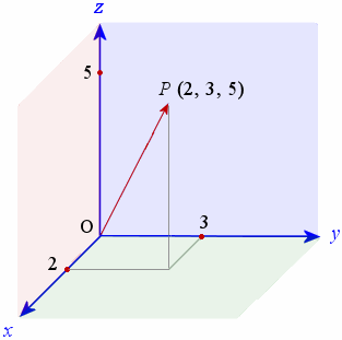
Here’s a practical example of how vectors work in 3D graph paper (Euclidean) space. Imagine I give you a spaceship that lets you fly in any direction, a starting point, and these instructions: go 2 miles along x, 3 miles along y, and 5 miles along z (relative to the starting point). These directions represent the change in coordinates that will take you from start to goal. The figure below shows this. You could get to the goal by going in the x direction, then the y direction, then the z direction, or by going in the z direction, then the x direction, then the y direction, or any combination of the three directions in any order. You could also go in a straight line to the goal coordinates. That straight line path is the vector and it would be defined by the distance that you had to travel along each axis to get from the start position to the final position.
Euclidean Distance Metrics
If you took the most direct path, you might be curious about the total distance that you traveled to get there (maybe your spaceship only has so much fuel or something). So how do you measure the distance along that most direct path?
There are two people who lived a long time ago who figured out the answer to that question. Both were Greek, one was named Euclid (the guy that Euclidean space is named after) and the other was named Pythagoras (the guy that the Pythagorean Theorem is named after). The distance between the two points along that vector we followed is called the Euclidean distance and it is a more general version of the Pythagorean Theorem. You could also say the Pythagorean Theorem is a special 2D case of the Euclidean distance metric.
The Pythagorean Theorem tells us that
$$a^2 + b^2 = c^2$$
and if we realize that a and b (the short sides of the triangle) are perpendicular to each other and could really be thought of as the x and y axes of our 2D space then we can write this as
$$x^2 + y^2 = c^2 = d^2$$
where c = d is the distance we traveled. Pretty cool huh.
In 3D (and higher dimensions) this also works. The distance we traveled in our spaceship is
$$x^2 + y^2 + z^2 = d^2$$
This can become a lot to write when we start getting to higher dimensions so we use linear algebra shorthand usually. We write our vector, v, as a list of numbers comprised of our directions in space
$$\mathbf{v} = \begin{bmatrix} x & y & z \end{bmatrix}^\top$$
and then we multiply the vector by itself using the dot product to get the same result as before
$$ x^2 + y^2 + z^2 = \mathbf{v}^\top \mathbf{v} = d^2$$
This means that we can now find the distance along any vector in any dimension of our graph paper (Euclidean) space. But what about on our globe? How do we find the distance between things there?
Riemannian Distance Metrics
The big issue with distance on our Riemannian manifold (think globe) is that it’s curved…this means that our standard linear algebra tools that we’ve been using to measure distance between points doesn’t work well in this space. If we tried to use these tools to measure distance using this vector math then that would be like cutting through the center of the earth to get from A to B rather than moving along the surface. The distance we calculated wouldn’t be accurate at all.
Fortunately we can get around that issue using linear algebra as well. If you look around you, it’s usually pretty hard to see the curvature of the earth. Things seem pretty flat. If they didn’t, the whole flat-earth theory would have never gotten any traction. If you were an ant then things would be even more different. To you, the idea of the earth being round would have no significant impact on how far you had to travel. Your paths would be so short that the distance if we pretended the earth was flat and the actual distance would functionally be the same.
We can exploit this fact to measure distances on the manifold. We assume that for every point (i.e. set of coordinates), \( \mathbf{x} \), on the manifold there is some matrix (a box of numbers),
$$\mathbf{M}(\mathbf{x})$$
that scales and shrinks the different dimensions of the space so that they are all equivalent. If we stick this box of numbers in the middle of our distance calculation like so
$$\mathbf{v}^\top~\mathbf{M}(\mathbf{x})~\mathbf{v} = d^2$$
then we have a good local approximation of distances around the point of interest x. We call this equation our Riemannian Distance Metric because it helps us measure and define distances on the Riemannian manifold.
Here’s an example of what this could look like in practice. Say the matrix is
\[ \mathbf{M}(\mathbf{x}) = \begin{bmatrix} 2 & 0 & 0 \\ 0 & 3 & 0 \\ 0 & 0 & 4 \end{bmatrix} \]
and \( \mathbf{v} = \begin{bmatrix}x & y & z\end{bmatrix}^\top \). The distance calculated at that point would be
$$\mathbf{v}^\top~\mathbf{M}(\mathbf{x})~\mathbf{v} = 2x^2 + 3y^2 + 4z^2 = d^2$$
Again, this distance squared would be the local approximation of the distance at that point. As long as v, the vector measuring the Euclidean (graph paper) distance between A and B, is small enough (think ant scale) then this is a good enough approximation. If A and B are far apart this is ok, we can deal with this. What we do is just break our long line into lots of small ant sized lines, compute the local approximations of the distance of each of those ant sized lines, and then add them all up to get the total distance. This is where knowing how to get a computer to do math for you becomes really helpful. No one wants to do that calculation by hand.
This is just an example, but it helps illustrate the point that I want to make. That Euclidean distance metric that we discussed earlier is actually a special case of the Riemannian Distance Metric. It’s like those Russian nesting dolls that fit inside each other. The Pythagorean Theorem is a special case of the Euclidean distance metric which is a special case of the Riemannian distance metric. Math is pretty cool that way.

Recap
Today we learned how to measure distance in SE(3) space, which is the space that our poses live in. We also learned what a pose is and that poses that seem close together in graph paper (Euclidean) space can actually be very far apart in SE(3) space. We also saw the idea of a Riemannian manifold for the first time. We used the globe analogy to help us understand and we learned that in order to do math on the manifold we have to respect how we move along its surface, just like how we can’t cut through the center of the earth to get from point A to B but instead have to travel along its surface.
So we know that SE(3) is a curved space, but we really like doing math on flat graph paper because it’s what we know best. What if I told you there’s a way to take any point on our globe, lay a perfectly flat piece of graph paper completely tangent to it, and do all our standard, comfortable vector math right there? In the next post we’re going to discuss how we can take all our tools for doing math in graph paper space and apply them to this new, SE(3) space. It’s a pretty cool trick and it’s fundamental to a lot of the stuff that we do in robotics so I recommend staying tuned for that!